Apache Hudi: From Zero To One (6/10)

Demystify clustering and space-filling curves

Apache Hudi: From Zero To One

• Post 1: A first glance at Hudi's storage format

• Post 2: Dive into read operation flow and query types

• Post 3: Understand write flows and operations

• Post 4: All about writer indexes

• Post 5: Introduce table services: compaction, cleaning, and indexing

• Post 6: Demystify clustering and space-filling curves

• Post 7: Concurrently run writers and table services

In the previous post, we covered the concept of table service and discussed compaction, cleaning, and indexing. To conclude this topic, we will now delve into the remaining service - clustering.

Overview

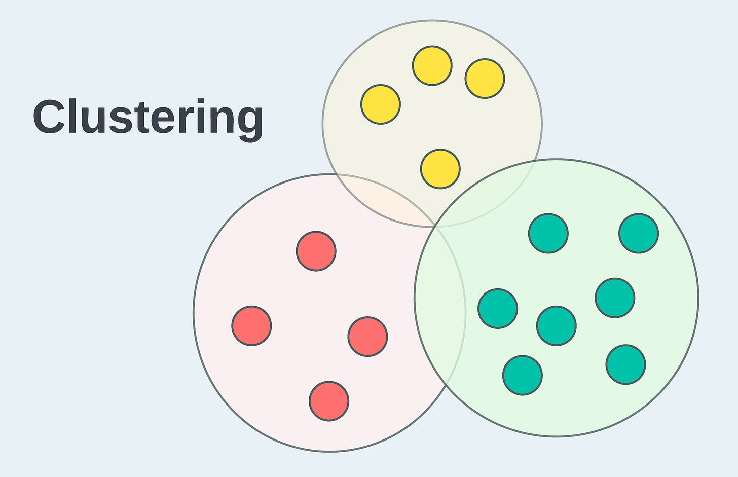
In the context of machine learning, clustering is a technique used to categorize data points into groups, unveiling underlying structures within the dataset. Many clustering algorithms employ specific methods to measure distances between data points, thereby determining the groups they belong to. When talking about clustering within the data storage domain, we can consider records as the data points and physical files as the groups. Therefore, the clustering process can be viewed as putting "proximate" records into the same files. You might naturally pose two follow-up questions: a) How can we determine if records are "proximate"? b) Why is clustering necessary?

To illustrate the concept of "proximity", let’s use the analogy of a 2-dimensional plane with X and Y axes. In this analogy, if a dataset’s schema has two columns, X and Y, and the records will be considered "close" when the value pairs (X, Y) are close to each other on the 2D plane. In case of wide schema with numerous of columns, more dimensions should be added accordingly. While visualizing high-dimensional spaces is challenging for 3-dimensional beings like ourselves, the proximity can still be determined mathematically, allowing computers to process the information.

Clustering, in the context of data storage, stands as a valuable optimization technique to improve the storage layout by preserving data locality for better read efficiency. There are three main motivations to perform clustering:

• Low-latency high-throughput writes often result in too many small files, hurting the query performance. A clustering task that consolidates and rewrites these data files into larger ones can effectively address the issue, especially when executed asynchronously to the writer.

• During the process of rewriting data files, "proximate" records are more likely to be clustered in the same files, thereby facilitating data-skipping techniques. Clustered records tend to show better alignment with the file-level statistics like column min/max values, allowing data files to be skipped more effectively based on given predicates.

• Reading clustered data can also take advantage of cache systems. The principle of spatial locality suggests that, following the access of certain data elements, nearby data elements are likely to be accessed in the near future. As clustered data exhibits good locality, utilizing block cache (e.g., in HDFS) can increase the hit rate, resulting in faster reads.

Clustering Workflow

Similar to other table services mentioned in post 5, clustering can be run in three modes: inline, semi-async, and full-async. Users are encouraged to consult the official documentation and configure these flags to control the running mode as needed.

hoodie.clustering.inline
hoodie.clustering.schedule.inline
hoodie.clustering.async.enabled

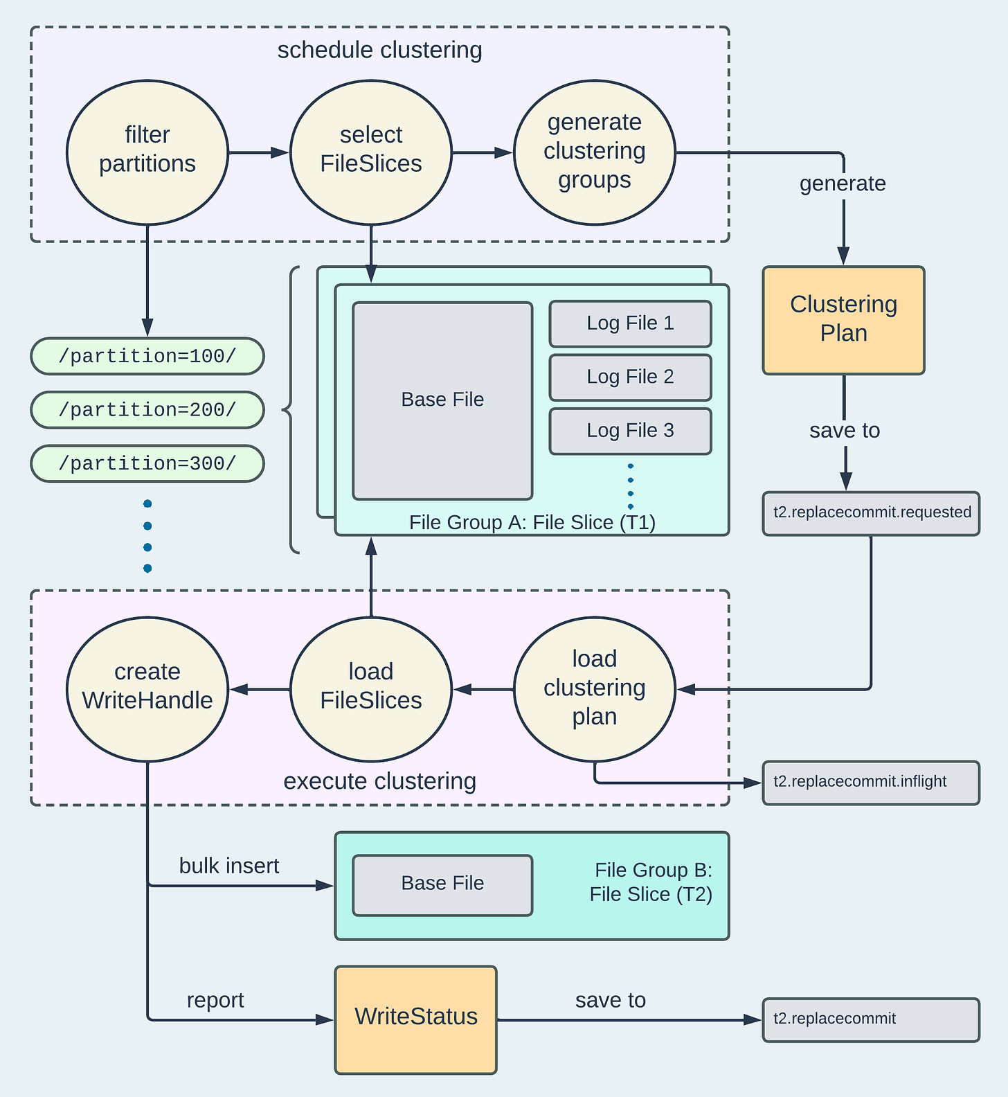
Since clustering involves rewriting data, a .replacecommit will be generated upon the completion of the table service job, indicating that the eligible File Groups have been rewritten into new ones. The clustering workflow, consisting of scheduling and execution, is illustrated below.

Hudi clustering workflow

The clustering workflow is akin to compaction. During the scheduling phase, eligible partitions and File Slices are selected based on ClusteringPlanStrategy. Users have the flexibility to define partition patterns (e.g., using Regex) to target specific partitions. Within these partitions, File Slices meeting certain criteria - such as not undergoing another pending compaction or not qualifying as small files - are added to HoodieClusteringGroups. These entities store information about the input and output for subsequent clustering execution. Typically, HoodieClusteringGroup adheres to size limits, such as the maximum total bytes of File Slices to include for rewriting. The total number of HoodieClusteringGroups is also capped by default, preventing unintentional submission of resource-intensive clustering jobs.

The execution phase involves high-level steps as below:

• Deserialize the clustering plan

• Load the designated input File Slices

• Merge the loaded records

• Bulk Insert the merged records to new File Groups

• Report write statistics through the returned WriteStatus

Users can customize the execution by supplying their own implementation of ClusteringExecutionStrategy. By default, each HoodieClusteringGroup defined in a clustering plan will be submitted as a separate job to perform parallel rewriting of File Slices.

For File Groups undergoing a clustering process, writers will, by default¹, abort if updates or deletes on those File Groups are intended. However, failing writes in the case of running table services may not be ideal. Other pluggable strategies exist that allow updates to proceed, followed by resolving conflicts or enforcing dual-writes on both the old and new File Groups.

We have illustrated how the clustering workflow looks like as a Hudi table service. However, one crucial piece of information was missing: where does the record "proximity" we mentioned in the overview come to play during the process? This occurs at the Bulk Insert step, where records are re-partitioned and sorted according to hoodie.layout.optimize.strategy, which I’ll elaborate on in the next section.

Space-filling Curves

Hudi offers three layout optimization strategies, namely Linear, Z-order, and Hilbert. Each of these defines how records should be sorted during Bulk Insert. The default strategy is Linear, which performs lexicographical sorting. The other two, Z-order and Hilbert, are known as space-filling curves that sort and preserve good spatial locality.

The Linear strategy is highly effective for datasets where record "proximity" relies on just one column. For instance, consider a table containing transaction records with a timestamp column. Analysts, for most of the time, run queries to fetch all records between transaction time A and B. Given that the records are considered "close" as long as the transaction timestamps are close, Linear is a perfect strategy due to sorting by the timestamp significantly preserve the locality.

The Linear strategy may not perform well with datasets that require two or more columns to determine record "proximity". Take, for example, a house inventory dataset with columns for latitude and longitude. Lexicographical sorting of latitude followed by longitude would group geographically distant house records together simply based on the proximity of latitude. In such cases, sorting algorithms capable of handling N-dimensional records are needed.

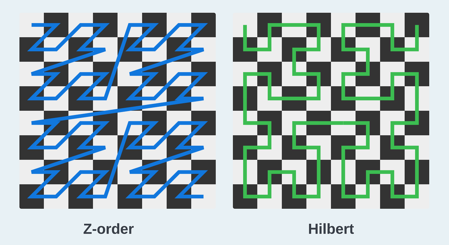
Space-filling curves are specifically designed to map N-dimensional points to one dimension. The term "space-filling" originates from the process where a curve traverses through the space, hitting all the possible points to fill it. Once the curve is straightened, all the multi-dimensional points are mapped to a one-dimensional space and assigned a single-value coordinate. Among various curve-drawing methods, Z-order and Hilbert, as shown below, are two approaches that can effectively preserve spatial locality through this mapping - the majority of nearby points on the curve are also close to each other in the original space.²

Z-order and Hilbert curves in 2D plane; credits to eisenwave.github.io

When we treat records as multi-dimensional points, drawing a Z-order or Hilbert curve essentially defines the way to sort them. Given that spatial locality is well preserved, actual "nearby" records are more likely to be stored in the same files. This fulfills the proximity condition explained in the overview and enhances read efficiency.

Recap

In this post, we completed the topic of table services by elaborating on clustering. Additionally, we discussed the space-filling curves and how they are used in the clustering process to optimizes the storage for reads. Please feel free to share your feedback and suggest content in the comments section.

Apache Hudi has a thriving community - come and engage with us via Slack, GitHub, LinkedIn, X (Twitter), and YouTube!

1. This behavior is controlled by hoodie.clustering.updates.strategy. Users may supply a subclass of org.apache.hudi.table.action.cluster.strategy.UpdateStrategy.

2. The Z-order curve has big jumps, indicating that some adjacent 1D points could actually be far away from each other in the original space. The Hilbert curve may perform better in preserving locality due to the absence of such cases.